Two fundamental difficulties in 20th century physics and ways to overcome them

What is the Physics?

Any description of physical system is an idealization, it is a correct (reasonable) abstraction from unimportant details to build a working model of the observed system. Obviously, no complete system can be described in all details. It is technically impossible, and unnecessary. Therefore, the physicist’s task can be briefly formulated as follows:

What should a physicist do?

1) Look at the object (system) and see all the interactions (of course, within the framework of existing modern knowledge).

2) Evaluate all the interactions seen, understand which ones and why can be “excluded” from consideration (from the model), and which interactions are significant and should be considered in the model.

3) Reasonably exclude everything unnecessary, leaving only the essential components, i.e. create a model describing the system (write out the equations of motion describing the model).

4) Compare the model with the experiment and, if necessary, improve it.

This is approximately how theoretical physics was organized until the first quarter of the 20th century. However, with the development of quantum mechanics, the approach to research has changed dramatically. Namely, the axiomatic approach has gained great popularity, in which all physical models began to be built on postulates / axioms and, sometimes, even on unfounded assumptions. In fact, axiomatic construction is recognized today as a norm and standard, although it has a serious drawback, since within its framework we do not see the foundations of the model (an example that immediately comes to mind is quantum mechanics). The number of postulates / axioms is huge, and we often do not even remember their existence, but simply take previously obtained results (based on axioms), introduce new postulates and obtain some formulas, which we compare with the experiment. Obviously, this path is a thoughtless enumeration of an infinite number of possible options, in the hope of guessing the correct equations. Moreover, as a rule, the original postulates and axioms are not even mentioned in modern articles, which is difficult to consider satisfactory.

Among these numerous postulates, there is one that is not usually remembered, since it is always assumed to be fulfilled a priori. We are talking about the postulate of completeness (closedness) of the system under consideration (which at first glance is obvious). However, in two key cases for modern physics, this postulate turned out to be unfulfilled, which led to serious complications.

At the very beginning of the 20th century, physicists faced two difficulties:

Astrophysicists faced the problem of the “non-physical” motion of observed objects.

Physicists faced the problem of explaining the line spectra of atoms.

Let’s see how the search for a way out of the impasse was carried out in the first and second cases.

Astrophysicists (left):                                                               Physicists (right):

Initially, in both cases, the task was: Find a description of the complete model of the system. The complete system looks like this:

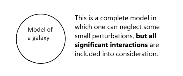Fig. 1.a. It is necessary to find a description of the dynamics of galaxies (it is necessary to construct a dynamic model that describes the observed rotation curves)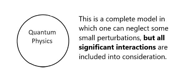

Fig. 1.b. It is necessary to explain the line spectra of atoms (it is necessary to construct a dynamic model of the radiating atom)

Schematically, we can distinguish parts of the systems under discussion (by place of dominance, as in galaxies, or due to the impossibility of correct accounting, as in an atom).

The system “by chance” (I emphasize once again – not by the will of physicists!) is unnaturally divided into two parts: “obvious” and “unknown”.

What do they do next in this case?

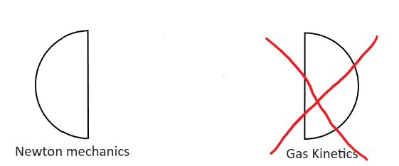Fig.3.a. Astrophysicists (without proving their assertion) say that gas kinetics are not important and they throw it out of consideration. However, in fact, elementary estimates (see the first part of the article, or preprint) show that gas kinetics dominate over gravity at large distances from the center of the galaxy, and therefore it cannot be neglected!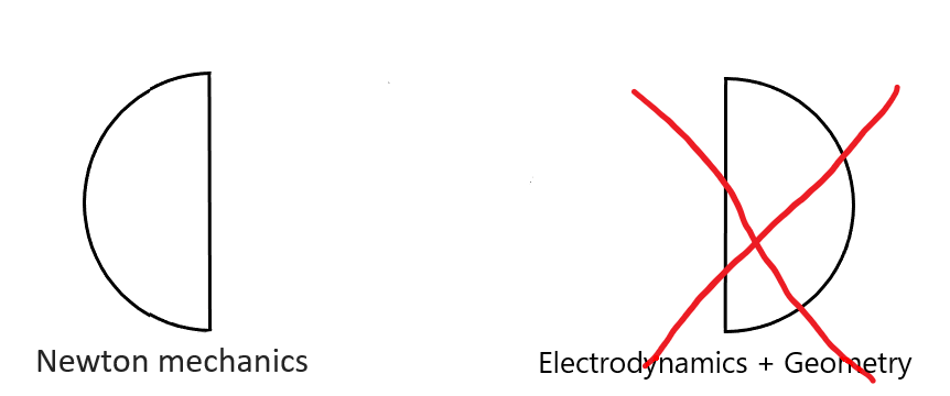

Fig.3.b. Physicists do not notice the bounded transverse EM field and do not know (let me remind you – it was 1926) that the Universe is expanding (see also the detailed comment* below). Willy-nilly, they have to look for a description (model) only of what is visible experimentally (the left half of quantum physics), which was successfully done by Schrödinger.

And now we have come to the most interesting part, namely to the question: How exactly were the models of incomplete, non-closed systems built in the first and second cases? In other words: how were the missing equations in the model compensated so that the remaining incomplete equations would describe the system under consideration?

Let’s take a look:

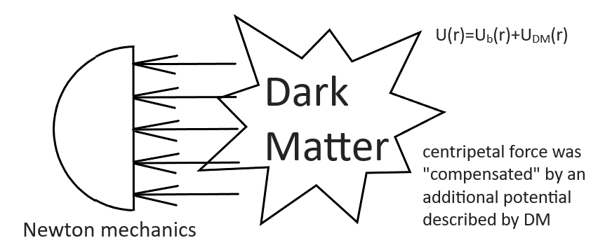Fig.4.a. Astrophysicists use only the equations of Newtonian mechanics and, in order to compensate for the problem (to adjust the calculations to the observations), they introduce a kind of “crutch” into the OLD Newtonian equations – an additional potential caused by an unobservable entity (some Dark Matter). In fact, several additional parameters were introduced into the incorrect, incomplete model to adjust the incorrect model to the observations. However, this manipulation did not help. Everything still remained crooked, askew and does not coincide with observations.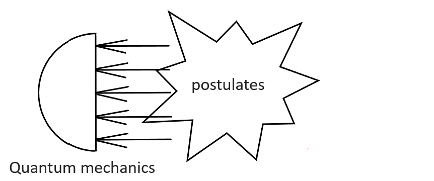

Fig.4.b. Physicists acted correctly (more carefully). They did not introduce some new unobservable entity to adjust the model to the experiment. They agreed that they do not know something essential about nature, and postulated NEW equations, which in essence were mechanics, however not usual, but “abnormal”, new (quantum) mechanics, based on postulates.   I repeat once again: The equations of quantum mechanics (Schrödinger equation, Klein-Gordon-Fock equation and Dirac equation) were postulated (guessed).

The physicists acted correctly, but the astrophysicists acted not quite right.

In the first and second cases, incomplete models were considered, but astrophysicists postulated an invisible, unobservable entity (DM), which is a gross error. At the same time, physicists agreed that they did not know something essential and simply introduced the necessary postulates into the basis of a new model (new equations). But they did not introduce a new entity such as “Quantonium matter”, that would correct Newton’s equation and mysteriously explain the quantization of atom within the framework of Newtonian mechanics. In Quantum Mechanics (QM) physicists took the right way, in astrophysics – not.

As a result:

Astrophysicists came to a fake science about the “properties and nature of DM”, which for a hundred years of existence led astrophysics and cosmology to a dead end. Only in 2023, with the receipt of the JWST results (which showed that the postulated dark matter does not fit into the observed reality at all) the first cautious publications against dark matter began to appear in journals.

Physicists got their hands on a correctly working model (quantum mechanics), but inevitably returned to the need to search for the meanings, foundations and origins of QM. They returned to need for an complete theory. Let me quote the classics:

“I do not like [quantum mechanics], and I am sorry I ever had anything to do with it.” (Erwin Schrödinger)

“I think I can safely say that nobody understands quantum mechanics.” (Richard Feynman)

“Quantum mechanics makes absolutely no sense.” (Sir Roger Penrose)

“Conventional formulations of quantum theory, and of quantum field theory in particular, are unprofessionally vague and ambiguous. Professional theoretical physicists ought to be able to do better. Bohm has shown us a way.” (John Bell)

______________________comment___________________

*(my comment). The fact that theorists did not assume that the Universe is expanding was correct. It would have been wrong in 1926 to include the expansion of the Universe in the QM or Maxwell equations. At that time, no one even guessed that the Universe is expanding. But the fact that they did not notice the transverse EM field, – was a clear mistake. They could have guessed this. However, let us note that at that time they were looking specifically and exclusively for the mechanics of atom. They believed that the photon appears only at the moment of emission, whereas before the photon does not exist, which is not entirely true. In fact, the “rudiments” of the photon are present before emission, but they look somewhat different. Ginzburg writes about this (not yet emitted) photon in his book “Astrophysics and Theoretical Physics. Additional Chapters”. Ginzburg calls it a “virtual photon” – this is a photon that has not yet been emitted, but definitely can be emitted. This is partly correct, but unfortunately, on the one hand, only partly, and on the other hand, this term is already used in QFT and its use can lead to confusion. I think it is more correct to call this EM field “coupled transverse EM field“.

The electron, “dangling” in orbit, generates the coupled transverse EM field, which is associated with the electron (here we need to remember the Bohm pilot wave: this is exactly what it is – a transverse EM wave is bounded with the electron. It was discussed in the article “the nature of quantum potential“). When the electron passes to a lower orbit, the boundary conditions imposed on the system by the external environment make it possible to emit a real photon (into which part of this “virtual” photon also passes). Part of this transverse EM energy (generated by the movement of the electron) is converted into a photon, which is emitted.

Let’s look at an analogy. It’s not entirely true, but this analogy is clear and easy to understand.

We see a lake and a ball in the water. When the ball is stationary (an isolated electron), there are no waves. However, in an atom, the electron is not isolated, but dangles around the nucleus. We start to “dangle” the ball in the water. It generates waves around itself. If these waves were quantized (like transverse EM waves – they are quantized due to the adiabatic expansion of the metric and the need to satisfy the boundary conditions), they would not diverge from the ball. Well, for example, let’s imagine that we do not have water but jelly. We select the elasticity of the jelly and the Boundary Conditions (BC) (the shape of the coastline and the bottom) in such a way that the propagation (departure) of the wave is damped. Then we would get this – we dangle the ball, and it generates waves that do not go to infinity (the equation of motion + BC do not form outgoing waves). Let’s call these waves “standing”. In Ginzburg’s book they are called “virtual photons” (not to be confused with virtual photons introduced into QED and QFT!). Now we will change the equations of motion, i.e. we will make such a motion of the ball that the boundary conditions are satisfied in the case of an outgoing wave (this is not just any motion, but a very specific one – an analogue of the transition of an electron from one orbit to another). This should be such a “tricky” motion that in combination with the boundary conditions it would be possible to tear off part of the “standing” wave. In this case, part of the energy of the ball and part of the energy of the “standing” wave “tear off” in the form of a “soliton” – in the form of a quantum, and are carried away to infinity.

(Attention!) The proposed analogy is not entirely accurate, since

1) There is a difference in speeds, which is significant for the physics of the processes under consideration (the speed of light is something special, related to the properties of the metric).

2) The signal transmission is different. In water – longitudinal, and for light – transverse.

3) There are dissipative losses in the example (which are not present in the electrodynamics of atom)

_________________End_of_comment__________________

What should we do now?

As you can see from Fig. 4, in the first case (4a) we have only one option – to finish the games with DM and just honestly write out all the equations describing the full system. This was done in 2018 and published in 2022. (see preprint)

In the second case (4b) there is no need to break anything, but simply consider the complete system and understand where the postulates came from. That is, finally find the foundations of quantum mechanics and complete the model to describe the complete system. It is in this case that QM is united with GR into a single, unified theory that Einstein dreamed of.

To do this, we should:

1) Realize that the transverse EM field (both free – “photon” and bounded in the atom “pilot wave”) should “feel” the change in the metric of space (a hint in this case is the observed cosmological redshift – i.e. “photon” = “transverse EM field” does not conserve its energy because of the expansion of the Universe, its energy-momentum is not an integral of motion).

2) Calculate the adiabatic invariant of the EM field ET=h, which is equal to Planck’s constant (see, for example, the first volume of Landau and Lifshitz, section “adiabatic invariant”). That is, in fact, the transverse EM field “feels” the expansion of the Universe!

3) Take the second volume of Landau and Lifshitz (where the equations of electrodynamics are derived from the principle of least action on a STATIONARY manifold), plus take a textbook of differential geometry, which shows how exactly the principle of least action is modified if the manifold is NOT stationary (i.e. the Universe is expanding). Combine this and obtain the equations of Complete Electrodynamics, which describe all areas of physics from quantum mechanics to relativistic electrodynamics, and also (as it should be) turn into Maxwell’s electrodynamics, in the limit of Planck’s constant tending to zero (the classical case).

The resulting equations provide: (1) a description of an atom (and any micro-system in general: classical, quantum, relativistic), (2) a cosmological red shift, (3) the Aharonov-Bohm effect, which the best minds have been struggling with unsuccessfully for many decades (see for example references in articles 1 and 2).

Thus, “Maxwell’s Electrodynamics” + “Quantum Mechanics” + “Relativistic Mechanics” were unified. All this has now become “Complete Electrodynamics“.

What Stephen Hawking and Sir Roger Penrose argued about so heatedly (unification of QM and GR) has become a reality.

Below, for convenience, a diagram is provided so that the relations between the topics and areas of physics are clear.

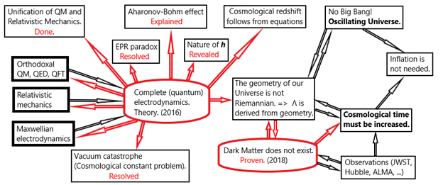
The red frame with smoothed corners highlights the published results. The Complete electrodynamics is published in this paper. The proof that dark matter does not exist is published in this paper. Black arrows go from the red frames – these are proven and published consequences. Thus, “orthodox QM, QED and QFT” + “Relativistic mechanics” + “Maxwell’s electrodynamics” (3 rectangles on the left) were combined into a single theory (Complete Electrodynamics). The unification made in the article is shown by red arrows.

Important: From the obtained “complete electrodynamics” follow all the equations from the three above-mentioned left rectangles (the main sections of modern physics: Electrodynamics, QM and GTR), as the corresponding limits. In this way it was possible to get rid of the postulates originally embedded in quantum mechanics (see, for example, the work).

Moreover, from Complete Electrodynamics follow:

– Solution to the EPR paradox, since the axiomatic introduction of wave functions (WF) is no longer required.

– The unification of QM and GR, since there is no more WF collapse.

– A natural explanation of the Aharonov-Bohm effect.

– The Planck constant is derived from geometry. In this case, quantum theory acquires meaning and foundation, and there is no longer a need for an axiomatic approach.

– The cosmological redshift is obtained naturally from the equations of electrodynamics.

– It is proved that the observed cosmological constant Λ has a geometric nature, which leads to a non-Riemannian geometry and agrees well with the latest JWST data.

– The problem of the vacuum catastrophe is resolved.

– Of course, all the equations used in QM are derived from Complete Electrodynamics (as it should be).

– In the limit h -> 0, the equations of Complete electrodynamics transform into Maxwell’s equations.

The consequence of the last two points is the complete agreement of the proposed theory with the entire experimental base accumulated in physics to date.

Thus, physics from a mosaic set becomes a whole unified theory. Moreover, as it turned out, the obtained equations of Complete electrodynamics are the equations of the Grand Unification. This is quite logical and expected, but we will talk about this later.